A simple example of resonance

In the climate change debate there is a faction that claims that the global warming we have experienced since approximately 1900 is due to changes in the sun's irradiance. The conventional wisdom among climate scientists is that since the solar irradiance varies only by 0.1%, solar irradiance variations are not powerful enough to bring about the observed temperature increases. However, Scafetta, West, Grigolini and others claim to have identified a stochastic resonance phenomenon that allows small variations to grow over time. Scafetta et. al.'s papers and analyses are quite challenging to follow. I am not convinced the climate change community is taking into account the resonance phenomenon. To demonstrate the potential of resonance to build up a large response from a small input I have put together a simple example using Mathematica. The example consists of a spring-mass system excited by a sinusoidal force at the resonant frequency. A small amount of damping is employed to keep the solution from growing too fast.

The system dynamics are given by
x'' + 2.0*delta*omegan*x' + (omegan^2)*x =b*omegan^2 +a*(omegan^2)*Sin[omega*t]

where x'' is the second derivative of x with respect to tim, and x' is the first.

Two runs were made. For both runs
omega = omegan = 10.0
delta = 0.001
b = 1.0
x'[0] = 0
x[0] = 1.0

For the first run a = 0.0. Thus the excitation is just a constant 1.0.

Here is a plot of the results of the first run



Note that since the excitation is the constant value 1.0, the output is the constant value 1.0
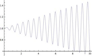
For the next run I set a = 0.001 - 0.1 percent of 1.0. Here are the results of the second run:


The addition of a 0.1 percent variation of the excitation makes a huge difference in the output.
A few comments are in order:

1. This is the simplest possible example. In no way do I intend to claim that this is what's going on in global warming. The point of the example is that a resonance in a system can lead to large swings of the system variables
2. Obviously for the resonance to occur, energy storage is required (the spring in our simple example) In the earth/sun system the energy storage may be in the oceans, the atmosphere, or eaven the earth itself
3. Scafetta suggests that one possible source of cycling of the earth' temperature is the wobble of the sun's position caused by the gravitational pull of the Jovian planets (Jupiter, Saturn)
   

References

1. Scafetta Talk at EPA:
   http://yosemite.epa.gov/ee/epa/eed.nsf/vwpsw/360796B06E48EA0485257601005982A1#video
2. Various publications on Scafetta's web site:
   http://www.fel.duke.edu/~scafetta/index-publications.html